Scripting Language Module
Scripting is a powerful way to extend the functionality of Tempas by controlling the simulation or processing of images in an automated way. One can create completely new algorithms to test out or implement new ideas
The scripting language for Tempas will be familiar to anyone who has ever created a program in C, C++ or has some experience with the scripting language for Digital Micrograph (copyright Gatan Inc.). In order to facilitate the creation of scripts for someone who has created scripts for Digital Micrograph, the scripting language has built in functions which will allow many DM scripts to be run without any (or few) modifications
To download the current Script Language Reference Manual, click HERE
Syntax Coloring has been added for easier readability and word completion adds to ease of use
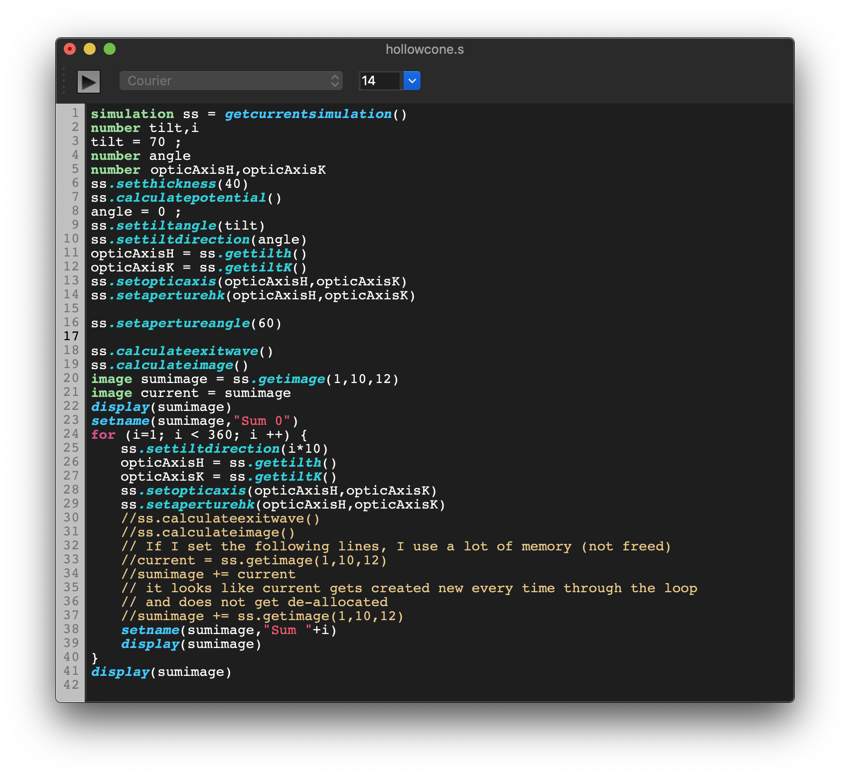
Examples: Digital Micrograph compatible scripts
Example 1:
Image test = newimage(“test”,512,512) // Creates a float image of size 512 by 512
test = exp(-iradius*iradius/100) // Fills the image with a gaussian with sigma = 10
display(test) // Displays the image
Example 1: Alternate Syntax - Non DM Compatible
Image test(512,512,exp(-iradius**2/100))
test.show()
// Displays the image
Example 2:
Image test = newimage(“test”,512,512) //
Creates a float image of size 512 by 512
test = sin(2*pi()*icol/8)+sin(2*pi()*irow/12)
// Fills the image with cross-fringes
// of period 8 and 12 pixels in x , y
display(test) // Displays the image
Example 2: Alternate Syntax - Non DM Compatible
Image test(512,512,sin(2*pi*icol/8)+sin(2*pi*irow/12))
test.display()
// Displays the image
Example3:
// Precession Tilt series
// This is summing over the power-spectrum of the exit wave function
// by spinning the beam in a circle. The beam tilt is theta (30 mrad).
// The increment in the azimuthal angle is dphi (6 degrees)
// A table of HKL values for different thicknesses is shown
// For illustration purposes, a precession image is also calculated
number theta = 30 // The tilt angle in mrad
number phi = 0 // Tilt angle (degrees) with respect to a-axis
number dphi = 6 // increments in tilt angle (degrees)
simulation sim = getsimulation() // Get the simulation
// We are making sure that everything has been calculated and is current
sim.calculateall()
Image xw = sim.loadexitwave() // Declare and load the exit wave
Image im = sim.loadimage() // Declare and load the image
Image sumim = im ; sumim = 0 ; // Declare the sum for the images and zero
Image sumps = xw ; sumps = 0 ; // Declare the sum for the powerspectrum
// and zero
Openlogwindow()
for(number thickness = 10; thickness <= 100; thickness += 10) {
sim.setthickness(thickness)
number i = 0 // declare and initialize our counter
for(phi = 0 ; phi < 360; phi += dphi) { // loop over the azimuthal angle
sim.settilt(theta,phi) // set the tilt of the specimen
// this is equivalent to the tilting the beam
sim.calculateexitwave() // Calculate the new exit wave
sim.calculateimage() // Calculate the new image
sumim += sim.loadimage() // Add the image to the sum
xw = sim.loadexitwave() // Load the exit wave
xw.fft() // Fourier transform to get the frequency
// complex coefficients
xw *= conjugate(xw) // Set the complex PowerSpectrum
// If we had used xw.ps() to get the
// power spectrum we would have had a real
// image in “real” space
sumps += xw // Add the powerspectrum to the sum
i++ // Keep track of the count
print("phi = "+phi) // Just to know where we are in the loop
}
sumim /= i // Divide by the number of terms in the sum
// Create a rectangular image of size 1024 by 1024 of sampling 0.1 Å (default)
Image precessionImage = sim.createimage(sumim,1024)
precessionImage.setname("Image Precession")
precessionImage.show() // Show the summed images
sumps /= i // Divide by the number of terms in the sum
sumps.sqrt() // To compare with the Scattering factors
// Create a rectangular image of size 1024 by 1024 out to gMax = 4 1/Å
// with a convergence angle of 0.2 mrad
Image precessionPS = sim.createfrequencyimage(sumps,1024,0.2,4)
precessionPS.setname("Power Spectrum Precession Thickness "+
sim.getthickness())
precessionPS.show() // Show the summed power spectrum
sumps.setname("thickness " + sim.getthickness())
sim.createhkltable(sumps)
}